Machine Learning

• AI > ML > Deep learning
  • AI: ability to learn by processing information, which will guide future processing abilities
  • ML: Ability to learn without explicitly being programmed
  • Deep learning: extract patterns from data using neural networks
• is learning from experience E, w.r.t. class of tasks T, performance measure P, if P improves with each E
• learning types: supervised, unsupervised, reinforcement, recommender system
• Singular or degenerate matrices don't have an Inverse

Concepts

• ML

  • Supervised: Classification, Regression
  • Unsupervised: Clustering (segmentation), Anomaly Detection, Association Rules (recommendation engine)

• Data types:

  • Qualitative:
    • Nominal: no ordering or ranking, e.g. Gender, Race
    • Ordinal: some ordering, performance, document security classification
    • Binary: True/False
  • Quantitative:
    • Discrete: quantities, number of children
    • Continuous: length, volume

Supervised

• algorithm is given a set of correct answers
• Regression: continuous (real-valued) output, eg: what's the value of my house?
  • curve fitting: linear, quadric
• classification: discrete output, eg: is it dog or a cat in the picture
  • features or attributes determine the output
• Model representation:`
  • training set: set of labeled data, consisting of \(m\) pairs of \(x\) input to \(y\) output $\((x,y)_{(i=1 \to m)}\)$
  • hypothesis: is a function that predicts value \(y\) based on input \(x\)
    • this is the output of the algorithm
  • linear regression: linear correlation between x and y
    • \(h(x) = \theta_0 + \theta_1 x\)
    • if x is just variable then it's called Univariate Linear Regression
  • cost function
    • Mean squared error function \(J_{(\theta_0, \theta_1)} = \frac{1}{2 . m} \sum_{i=0}^m (h_{\theta}(x^{(i)} - y^{(i)})^2\)

multi-variate linear regression

• when there is more than one feature
• feature scaling : every feature is scaled to have a value somewhere (not strict) in the range -1 and +1
  • helps gradient descent algorithm find minimum in a reasonable time
  • mean normalization : making all values scale between -0.5 and 0.5 (except x0) \(X_i = \frac{(X_i - M_i)}{S_i}\) where \(M_i\) is the average, \(S_i\) is the range for each feature i
• Number of features can be combined or expanded to suit the model, e.g.
  • if you have frontage and width of the house, then you can combine into one feature called area
  • if your feature isn't polynomial i.e. \(y = x + x^n...\), you can introduced each polynomial term as independent feature, thus converting polynomial regression to multi-variate linear regression.

minimizing cost function

Gradient Descent	Normal Equation
Need to choose alpha	No need to choose alpha
Needs many iterations	DIrect solution by solving
good whenn > 10,000	good when n is small

gradient descent

• is calculated as derivative of the above formula
  • learning rate (alpha) is the change that is applied to make cost function converge

normal equation

• allows you to solve for the minimize cost function.
  • since cost function is a quadratic function, solving for derivative of cost function = 0, will yield that value. In other words, solve for when the slope is zero (parallel to x axis)
• normal equation for a multi-variate function will involve solving for partial derivative of each variable.
• design matrix is a matrix of m samples by n+1 features
• since partial derivatives of multi-variate linear regression is complicated, use follow to find optimal value of theta (minimizes cost function): \(\theta = pinv(X^\prime * X) * X^\prime * y\), where \(X\) is the design matrix, \(X^\prime\) = \(X\) transposed, \(y\) is the value vector
• common causes of non-invertible matrices, i.e. ones that don't have an inverse (singular or degenerate matrices)
  • Redundant features or linearly dependent features: e.g. area in sq. ft. and sq. mt.
  • too many features: (m < n), delete some features or use regularization

Picking an ML Algorithm

Common classification models: - Logistic Regression: Binary classification - Simpler, used for establishing a baseline before trying more complex models - Naive Byes: high-bias, low-variance model - simple, low CPU usage, quick to train - if the data grows in size and variance, other models might work better - K-nearest-neighbor (KNN): classification by taking vote of K nearest neighbors, regression by taking mean of \(f\) value of K nearest neighbors - quick to train - easily fooled by irrelevant attributes obscuring important ones. - query time and storage grows rapidly for large datasets, because it requires training data to be kept around - decision tree: - main advantage is easy to explain how the results were achieved simply by following the path from root to the leaf node - they tend to overfit (can be mitigated by some techniques) - Support Vector Machine (SVM): used for problems with exactly two classes; finds a hyperplane that separates two classes such that the points in either classes are farthest from points in the other class - extremely accurate, less prone to overfit, - linear SVM are easy to interpret and fast - can handle complex, non-linear classifications by technique called kernel-trick - cons: speed is heavily impacted if there are more than two classes, requires upfront training and tuning - Artificial Neural Networks: - great for nonlinear data with high number of features (such as character recognition, stock market prediction) - con: hard to fine-tune, needs creating a new model with changed ata - con: computationally intensive - con: difficult explainability

Logistic Regression

• For binary classification, hypothesis function needs to be: 0 <= h(x) <= 1
• Sigmoid (aka Logistic) function = g(z), where z = (theta Transpose dot X)
• Decision boundary: A boundary that delineates probability that y=1 or theta-T X >= 0
• symmetry breaking: Assigning random values to initial parameters in neural network, so they can converge better
• One-vs-all: When selecting one of a class, instead of binary, e.g. weather is cold, rainy, sunny or hot,
  • Use logistic regression for each value of class (one v/s all)

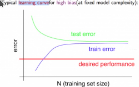
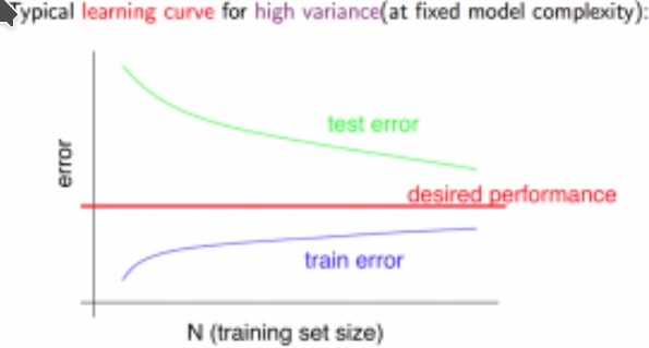
Over-fitting

• applies to both, linear or logistic regression
• High Bias: very simple graph such as linear, doesn't fit training set (samples) well. E.g. house price v/s size plateaus after certain size, which a straight line would predict that prices should go up proportionately with house size
• High Variance: A complex graph, usually high-order polynomial, that does fit the entire training set, for example a quadratic function of price v/s size, but it is too uneven and probably won't fit if we had a larger training set. Due to unevenness, this is called high variance
• Solutions:
• Reduce number of features: manually or model selection algorithm
• Regularization: keep all features, but reduce the magnitude of \(\theta_j\) if features contribute only marginally

Regularization

• penalize certain features by adding a high multiplier (lambda aka regularization parameter) in the cost function.
• by convention lambda is not applied to \(\theta_0\) (i.e. feature with constant value 1)
• Cost function is then made up of two goals: 1) fit the training sample 2) keep theta small
  • if lambda is too high, then it results in \(\theta_0\) being the only non-zero parameter,
    • i.e. no other features playing any part (because they are close to 0), i.e. straight horizontal line, i.e. under-fitting
• Regularization also solves the non-invertibility/singular (aka degenerate) problem encountered during normal equation when \(m < n\) (training set has fewer samples than number of features)
• normal equation with regularization: \(\theta = inv(X^\prime \cdot X + \lambda \cdot L) * X' *y\) where L is like an identity matrix, except top element of the diagonal is 0

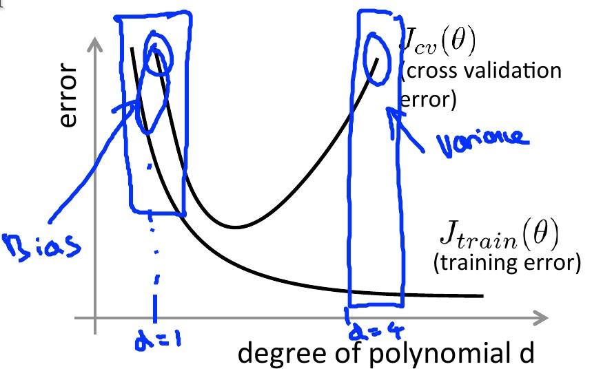
Diagnosing Algorithm Performance

• High Bias: under-fitting; High Variance: over-fitting
• ROT: split data into 3 sets:
  • Training set: data to train the model with, ~60%
  • (Cross) Validation CV: use for finding the best regularization parameter (lambda)
  • Test set: estimate generalization error using theta (d)

techniques for High ->	Bias	Variance
training samples		++
number of features	++	--
polynomial features	++
lambda (regularization)	--	++
neural network # of neurons/layers	++	--

• ROT: If you have a low-bias algorithm, using very high number of training samples will benefit the algorithm the most
  • If the answer to the question Can a human expert predict accurately based on given features? is yes, then algorithm is likely to be low-biased and will likely get a boost by using a larger training set

Stochastic Gradient Descent

• For large training set (in millions), optimize the batch (the default algorithm) gradient descent algorithm
• involves minimizing cost function using only one training sample during each iteration instead of the entire training set
• since theta calculation from just 1 training example can be misleading, iterate multiple training samples and average new theta value
  • ROT: if there may be local minimas (noisy cost function curve), increase number of training samples to smoothen it out
• may not reach global minimum
  • slowly decrease learning rate (alpha) with each iteration
• mini-batch gradient descent involves minimizing cost function using a small subset of training sample during each iteration
• online learning is a streaming learning where each data is used once to incrementally improve theta and then discarded

Error Metrics for Skewed Data

• Value 1 by convention is used for value that is rare/anomalous (eg patient with cancer)
• For skewed classification, eg if a patient has cancer (1) or no (0), traditional error rate doesn't give very accurate picture
  • eg. if error rate is 1%, but number of patients with cancer is 0.5% then we are off by half
  • Use Precision/Recall to measure skewed data.
• 
  • Precision: Of all positively classified cases how many are true positives: True Pos / (True Pos + False Pos)
  • Recall: of all true positives, how many were classified as positives: True Pos / (True Pos + False Neg)
  • Accuracy = (true pos + true neg) / (tot examples)
• Trade off between Precision and Recall
  • e.g. instead of h(x) >= 0.5 if choose h(x) >= 0.9 we'll achieve high precision, but low recall (most predicted cancer patient do actually have cancer)
  • high precision means lower recall (eg h(x) < 0.9 more patients will be predicted as not having cancer than true cancer patients)
• F Score : analytical way to choose between high precision or high recall algorithms. \(F = \frac{2PR}{P + R}\)

Unsupervised

• algorithm has no knowledge of results needed, tries to build a structure from a given dataset
• General types:
  • clustering: market segmentation, social networking, general cohesiveness
  • dimension reduction
  • anomaly detection
  • association

K-Means clustering

• Let,
  • K be the number of cluster
  • C be a cluster, with suffix from {1..k}
  • Mu be the Centroid of each cluster with suffix from {1..k}
    • centroids are initialized as randomly picking K samples
  • J be the cost or distortion
    • average of square of distance of each sample from the centroid of the cluster to which it is assigned
• Minimizing J involves two steps
  • cluster assignment: \(x_{(i)}\) is assigned to a cluster \(C_{(k)}\) whose centroid is closest to it
  • move centroid: pick a new centroid as a average of all points within the cluster
• Can have local maxima
  • for small values of \(m\), run algorithm
• Choosing \(K\) automatically
  • Elbow method involves picking \(K\) for which reduction in \(J\) is maximum

ML Pipelines

• A pipeline consisting of individual ML or non-ML steps
• E.g. OCR in an image consists of these steps
  • Finding text areas (using sliding window)
  • Segmenting characters within text areas (using 1D sliding window to find gaps between characters)
  • character recognition
• ceiling analysis
  • objective: in a complex pipeline, evaluate which component to work on to improve pipeline efficiency
  • evaluate pipeline efficiency, by providing ground-truth labels to components and pick the one that yields max improvements